06 · Datenbereinigung und Datentransformation
tidy_long_wide.svg
Abbildung · Quellcode
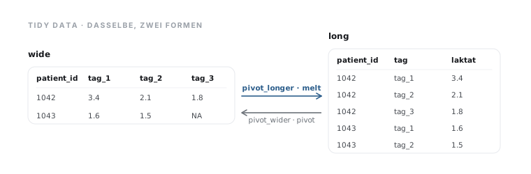
Erzeugt von tidy_long_wide() in lib/diagrams.py, Zeile 267–305.
Python
Python-Code: in eine Datei mit Endung
.py schreiben und mit dem ▶-Knopf in VS Code ausführen – oder Zeile für Zeile in die Python-Konsole. Setzt die in Modul 02 eingerichtete Umgebung voraus.def tidy_long_wide() -> str: b = [eyebrow(40, 40, "Tidy Data · dasselbe, zwei Formen")] # WIDE wx, wy = 40, 96 wide_head = ["patient_id", "tag_1", "tag_2", "tag_3"] wide_rows = [["1042", "3.4", "2.1", "1.8"], ["1043", "1.6", "1.5", "NA"]] cw = 74 b.append(txt(wx, wy - 14, "wide", size=12, fill=T["ink"], w=600, mono=True)) b.append(rect(wx, wy, cw * len(wide_head), 30 + 26 * len(wide_rows), r=10, fill=T["card"], stroke=T["rule"])) for j, h in enumerate(wide_head): b.append(txt(wx + j * cw + 12, wy + 20, h, size=10.5, fill=T["ink"], w=600, mono=True)) b.append(line(wx + 12, wy + 30, wx + cw * len(wide_head) - 12, wy + 30, stroke=T["hair"])) for i, r in enumerate(wide_rows): for j, v in enumerate(r): b.append(txt(wx + j * cw + 12, wy + 48 + i * 26, v, size=10.5, fill=T["ink2"], mono=True)) # LONG lx, ly = 470, 70 long_head = ["patient_id", "tag", "laktat"] long_rows = [["1042", "tag_1", "3.4"], ["1042", "tag_2", "2.1"], ["1042", "tag_3", "1.8"], ["1043", "tag_1", "1.6"], ["1043", "tag_2", "1.5"]] lcw = 82 b.append(txt(lx, ly - 14, "long", size=12, fill=T["ink"], w=600, mono=True)) b.append(rect(lx, ly, lcw * len(long_head), 30 + 24 * len(long_rows), r=10, fill=T["card"], stroke=T["rule"])) for j, h in enumerate(long_head): b.append(txt(lx + j * lcw + 12, ly + 20, h, size=10.5, fill=T["ink"], w=600, mono=True)) b.append(line(lx + 12, ly + 30, lx + lcw * len(long_head) - 12, ly + 30, stroke=T["hair"])) for i, r in enumerate(long_rows): for j, v in enumerate(r): b.append(txt(lx + j * lcw + 12, ly + 46 + i * 24, v, size=10.5, fill=T["ink2"], mono=True)) # Transform-Pfeile mx1, mx2, myc = wx + cw * len(wide_head), lx, 150 b.append(arrow(mx1 + 10, myc - 12, mx2 - 10, color=T["acc"])) b.append(txt((mx1 + mx2) / 2, myc - 20, "pivot_longer · melt", size=10.5, fill=T["acc"], w=600, anchor="middle", mono=True)) b.append(f'<path d="M{mx2-10},{myc+12} L{mx1+10},{myc+12}" stroke="{T["mut"]}" stroke-width="1.6" fill="none"/>') b.append(f'<path d="M{mx1+10},{myc+12} l7,-4 M{mx1+10},{myc+12} l7,4" stroke="{T["mut"]}" stroke-width="1.6" fill="none" stroke-linecap="round"/>') b.append(txt((mx1 + mx2) / 2, myc + 26, "pivot_wider · pivot", size=10.5, fill=T["mut"], anchor="middle", mono=True)) return canvas(760, 250, "".join(b), "Tidy Data: dieselben Laktatverläufe im wide-Format (eine Spalte pro Tag) und im long-Format " "(eine Zeile pro Messung); pivot_longer/melt und pivot_wider wandeln ineinander um.")