12 · Regressionsmodelle: Lineare, logistische und Cox-Regression
forest_odds_ratios.png
Abbildung · Quellcode
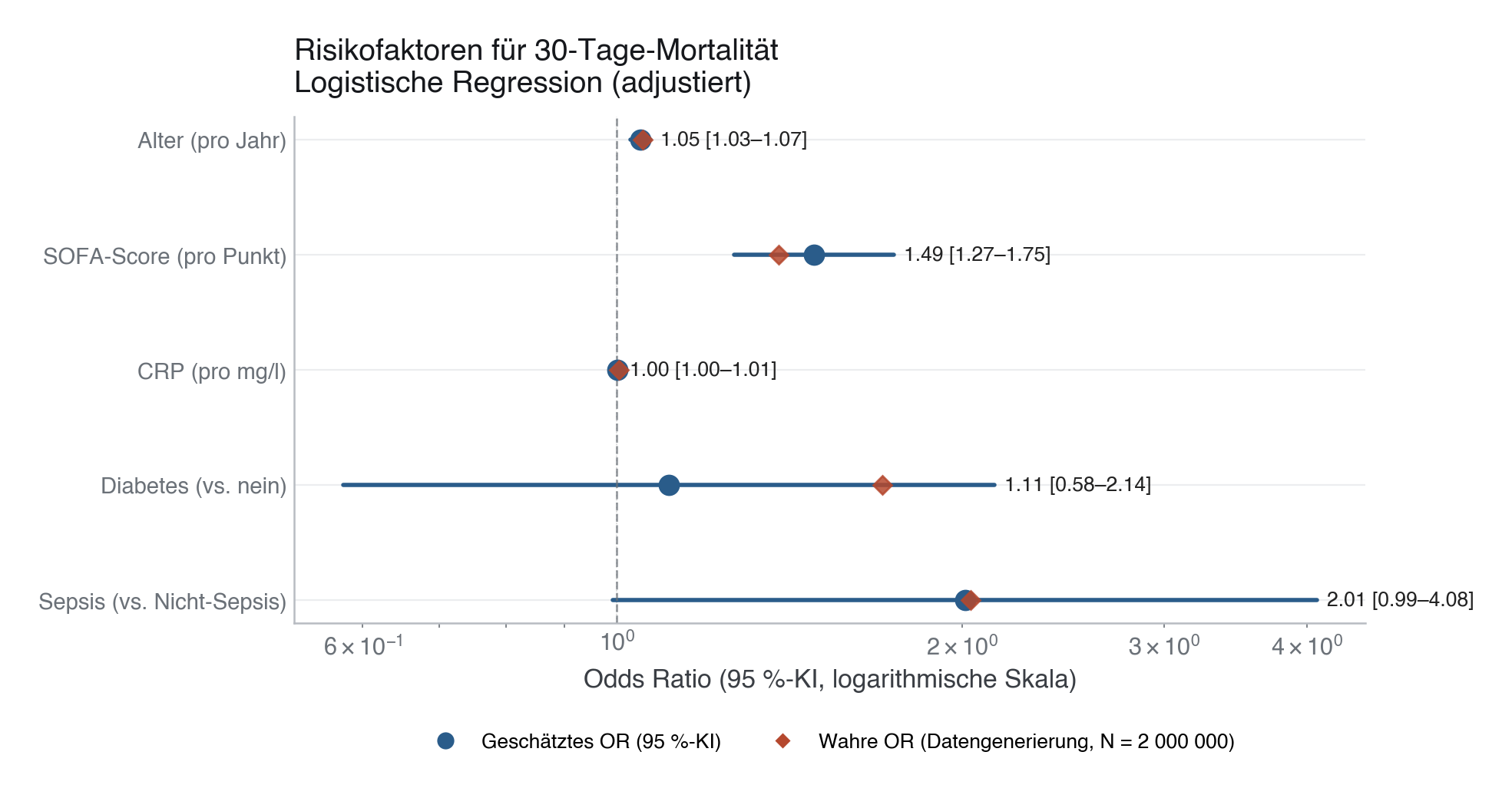
Erzeugt im Abschnitt „MODULE 12 · Forest plot: odds ratios + KM curve" in data/figures.py, Zeile 423–510.
Dieses Skript läuft von oben nach unten. Der gemeinsame Vorspann — Bibliotheken, Kohorte laden, Plot-Stil — steht am Anfang der vollständigen Datei und gilt für alle Abbildungen darin.
Python
Python-Code: in eine Datei mit Endung
.py schreiben und mit dem ▶-Knopf in VS Code ausführen – oder Zeile für Zeile in die Python-Konsole. Setzt die in Modul 02 eingerichtete Umgebung voraus.# =========================================================================== # MODULE 12 · Forest plot: odds ratios + KM curve # =========================================================================== print("[12] Forest Plot & Kaplan-Meier ...") import statsmodels.formula.api as smf cohort["aktiv_raucher"] = (cohort["raucherstatus"] == "aktiv").astype(int) cohort["sepsis"] = (cohort["aufnahmegrund"] == "Sepsis").astype(int) formula = ("verstorben_30d ~ alter + sofa_score + crp_mg_l " "+ diabetes + sepsis") model = smf.logit(formula, data=cohort).fit(disp=0) # OR and 95% CI params = model.params.drop("Intercept") conf = model.conf_int().drop("Intercept") or_est = np.exp(params) or_lo = np.exp(conf[0]) or_hi = np.exp(conf[1]) # True ORs for exactly this model specification. # # NOT exp(beta) from generate_data.py: those betas are log-HAZARDS of a Weibull # process, so exponentiating them yields hazard ratios. This plot shows odds # ratios, and at a 15.6 % event rate the true OR lies further from 1 than the # true HR. lib/ground_truth.py replays the generating process at N = 200 000 and # fits this same model to obtain them. true_or = true_odds_ratios_for(("alter", "sofa_score", "crp_mg_l", "diabetes", "sepsis")) # German display labels for predictors predictor_labels = { "alter": "Alter (pro Jahr)", "sofa_score": "SOFA-Score (pro Punkt)", "crp_mg_l": "CRP (pro mg/l)", "diabetes": "Diabetes (vs. nein)", "sepsis": "Sepsis (vs. Nicht-Sepsis)", } predictor_order = list(params.index) y_pos = list(range(len(predictor_order) - 1, -1, -1)) # reversed order fig, ax = plt.subplots(figsize=(9, 5)) for i, (pred, y) in enumerate(zip(predictor_order, y_pos)): est = or_est[pred] lo = or_lo[pred] hi = or_hi[pred] # CI line ax.plot([lo, hi], [y, y], color=PRIMARY, linewidth=2.0, solid_capstyle="round") # Point estimate ax.plot(est, y, "o", color=PRIMARY, markersize=9, zorder=5) # True OR (small diamond) if pred in true_or: ax.plot(true_or[pred], y, "D", color=EVENT, markersize=6, zorder=6, alpha=0.85) # Label: OR [CI] ci_label = f"{est:.2f} [{lo:.2f}–{hi:.2f}]" ax.text(max(hi, 1.0) * 1.02, y, ci_label, va="center", fontsize=9.5, color="#222222") # Reference line at OR = 1 ax.axvline(1.0, color=SECONDARY, linestyle="--", linewidth=1.0, alpha=0.7) # y-axis: variable names in German ax.set_yticks(y_pos) ax.set_yticklabels([predictor_labels.get(p, p) for p in predictor_order], fontsize=10.5) ax.set_xscale("log") ax.set_xlabel("Odds Ratio (95 %-KI, logarithmische Skala)") ax.set_title("Risikofaktoren für 30-Tage-Mortalität\nLogistische Regression (adjustiert)") # Grid on x-axis too ax.grid(axis="x", linestyle=":", linewidth=0.7, color="#DDDDDD") # Legend from matplotlib.lines import Line2D legend_items = [ Line2D([0], [0], marker="o", color="w", markerfacecolor=PRIMARY, markersize=9, label="Geschätztes OR (95 %-KI)"), Line2D([0], [0], marker="D", color="w", markerfacecolor=EVENT, markersize=6, label="Wahre OR (Datengenerierung, N = 2 000 000)"), ] ax.legend(handles=legend_items, loc="upper center", bbox_to_anchor=(0.5, -0.18), ncol=2, fontsize=9.5, frameon=False) fig.subplots_adjust(bottom=0.22) save(fig, ASSETS / "12-regression" / "assets" / "forest_odds_ratios.png")