12 · Regressionsmodelle: Lineare, logistische und Cox-Regression
residual_diagnostics.png
Abbildung · Quellcode
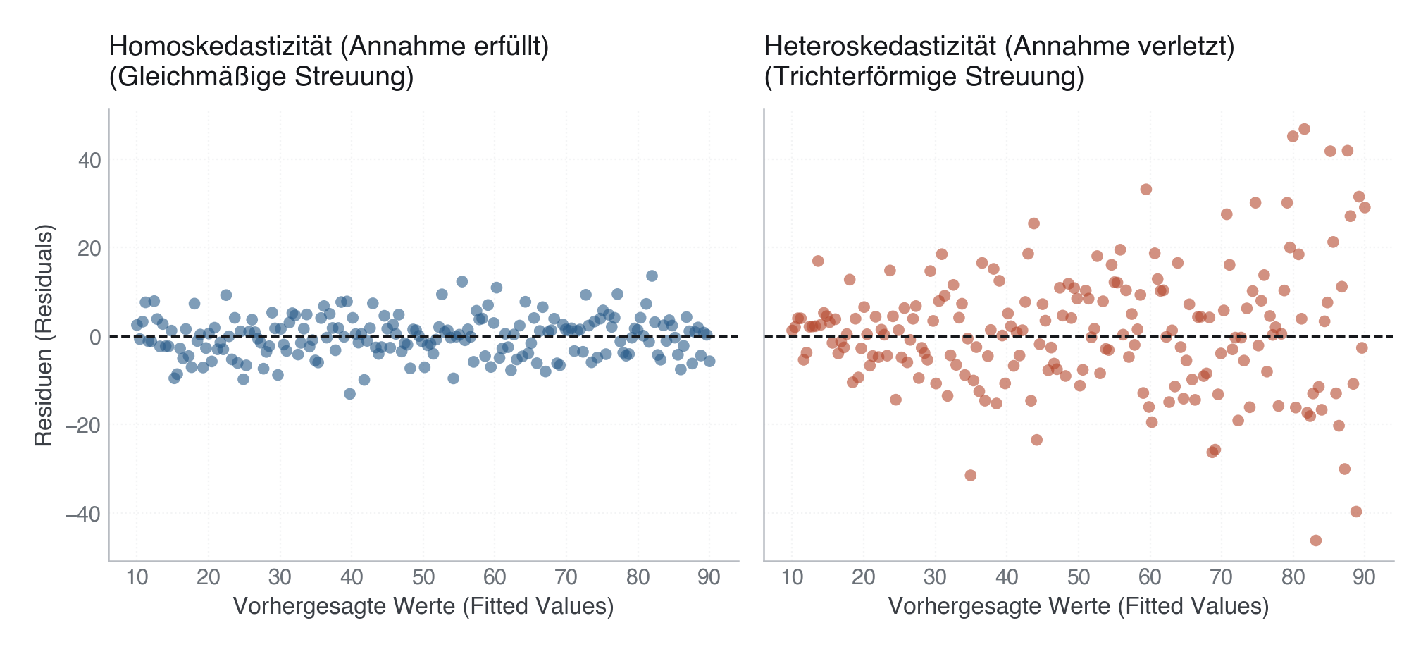
Erzeugt im Abschnitt „residual_diagnostics" in data/figures.py, Zeile 555–586.
Dieses Skript läuft von oben nach unten. Der gemeinsame Vorspann — Bibliotheken, Kohorte laden, Plot-Stil — steht am Anfang der vollständigen Datei und gilt für alle Abbildungen darin.
Python
Python-Code: in eine Datei mit Endung
.py schreiben und mit dem ▶-Knopf in VS Code ausführen – oder Zeile für Zeile in die Python-Konsole. Setzt die in Modul 02 eingerichtete Umgebung voraus.# --- Regression Residual Diagnostics --- print("[12] Regressions-Residuendiagnostik ...") np.random.seed(42) fitted_vals = np.linspace(10, 90, 200) # 1. Homoscedasticity (Good model): residuals are a constant band residuals_good = np.random.normal(0, 5, len(fitted_vals)) # 2. Heteroscedasticity (Violated model): variance increases with fitted values (funnel shape) residuals_bad = np.random.normal(0, 1.0 + 0.25 * fitted_vals, len(fitted_vals)) fig, (ax1, ax2) = plt.subplots(1, 2, figsize=(10, 4.5), sharey=True) # Homoscedasticity ax1.scatter(fitted_vals, residuals_good, color=PRIMARY, alpha=0.6, edgecolors="none") ax1.axhline(0, color="#16181C", linestyle="--", linewidth=1.2) ax1.set_xlabel("Vorhergesagte Werte (Fitted Values)") ax1.set_ylabel("Residuen (Residuals)") ax1.set_title("Homoskedastizität (Annahme erfüllt)\n(Gleichmäßige Streuung)") ax1.grid(True, linestyle=":", alpha=0.6) # Heteroscedasticity ax2.scatter(fitted_vals, residuals_bad, color=EVENT, alpha=0.6, edgecolors="none") ax2.axhline(0, color="#16181C", linestyle="--", linewidth=1.2) ax2.set_xlabel("Vorhergesagte Werte (Fitted Values)") ax2.set_title("Heteroskedastizität (Annahme verletzt)\n(Trichterförmige Streuung)") ax2.grid(True, linestyle=":", alpha=0.6) plt.tight_layout() (ASSETS / "12-regression" / "assets").mkdir(parents=True, exist_ok=True) save(fig, ASSETS / "12-regression" / "assets" / "residual_diagnostics.png")