15 · Kausale Inferenz und Directed Acyclic Graphs
kausale_dag.svg
Abbildung · Quellcode
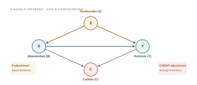
Erzeugt von kausale_dag() in lib/diagrams.py, Zeile 453–499.
Python
Python-Code: in eine Datei mit Endung
.py schreiben und mit dem ▶-Knopf in VS Code ausführen – oder Zeile für Zeile in die Python-Konsole. Setzt die in Modul 02 eingerichtete Umgebung voraus.def kausale_dag() -> str: import numpy as np b = [eyebrow(40, 40, "Kausale Inferenz · DAG & Confounding")] # Helper to draw node circle with text def node(x, y, label, col, bg): return (f'<circle cx="{x}" cy="{y}" r="26" fill="{bg}" stroke="{col}" stroke-width="1.8"/>' + txt(x, y + 4, label, size=14, fill=col, w=700, anchor="middle", mono=True)) b.append(node(150, 180, "X", T["acc"], T["acct"])) b.append(node(550, 180, "Y", T["ok"], T["okt"])) b.append(node(350, 90, "Z", T["warn"], T["warnt"])) b.append(node(350, 270, "C", T["death"], T["deatht"])) def arrow_line(x1, y1, x2, y2, color): dx, dy = x2 - x1, y2 - y1 length = np.hypot(dx, dy) ux, uy = dx / length, dy / length sx1, sy1 = x1 + ux * 28, y1 + uy * 28 sx2, sy2 = x2 - ux * 30, y2 - uy * 30 ax, ay = sx2 - ux * 8, sy2 - uy * 8 px, py = -uy * 5, ux * 5 head = f'M{sx2},{sy2} L{ax+px},{ay+py} L{ax-px},{ay-py} Z' return (line(sx1, sy1, sx2, sy2, stroke=color, sw=2) + f'<path d="{head}" fill="{color}"/>') b.append(arrow_line(150, 180, 550, 180, T["acc"])) b.append(arrow_line(350, 90, 150, 180, T["warn"])) b.append(arrow_line(350, 90, 550, 180, T["warn"])) b.append(arrow_line(150, 180, 350, 270, T["mut"])) b.append(arrow_line(550, 180, 350, 270, T["mut"])) b.append(txt(150, 222, "Intervention (X)", size=11, fill=T["acc2"], w=600, anchor="middle")) b.append(txt(550, 222, "Outcome (Y)", size=11, fill=T["ok"], w=600, anchor="middle")) b.append(txt(350, 48, "Confounder (Z)", size=11, fill=T["warn"], w=700, anchor="middle")) b.append(txt(350, 312, "Collider (C)", size=11, fill=T["death"], w=700, anchor="middle")) b.append(rect(40, 240, 96, 50, r=6, fill=T["warnt"])) b.append(txt(45, 258, "Z adjustieren!", size=10, fill=T["warn"], w=700)) b.append(txt(45, 276, "(blockt Backdoor)", size=9, fill=T["mut"])) b.append(rect(610, 240, 110, 50, r=6, fill=T["deatht"])) b.append(txt(615, 258, "C NICHT adjustieren!", size=10, fill=T["death"], w=700)) b.append(txt(615, 276, "(erzeugt Scheinkorr.)", size=9, fill=T["mut"])) return canvas(760, 330, "".join(b), "Causal DAG representation showing Confounder and Collider adjustment rules")