15 · Kausale Inferenz und Directed Acyclic Graphs
simpsons_paradox.png
Abbildung · Quellcode
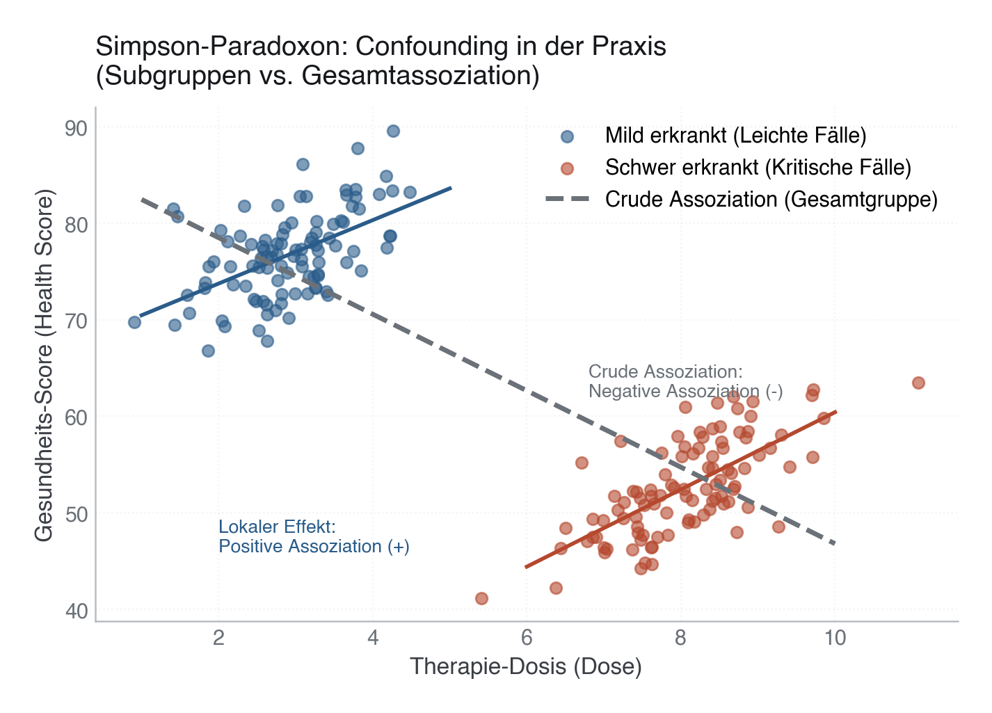
Erzeugt im Abschnitt „MODULE 15 · Causal Inference (Simpson's Paradox)" in data/figures.py, Zeile 625–672.
Dieses Skript läuft von oben nach unten. Der gemeinsame Vorspann — Bibliotheken, Kohorte laden, Plot-Stil — steht am Anfang der vollständigen Datei und gilt für alle Abbildungen darin.
Python
Python-Code: in eine Datei mit Endung
.py schreiben und mit dem ▶-Knopf in VS Code ausführen – oder Zeile für Zeile in die Python-Konsole. Setzt die in Modul 02 eingerichtete Umgebung voraus.# =========================================================================== # MODULE 15 · Causal Inference (Simpson's Paradox) # =========================================================================== print("[15] Kausale Inferenz (Simpson's Paradox) ...") np.random.seed(42) n_patients = 100 # Mild group: low dose, high health score dose_mild = np.random.normal(3.0, 0.8, n_patients) health_mild = 65 + 4 * dose_mild + np.random.normal(0, 4.0, n_patients) # Severe group: high dose, low health score dose_severe = np.random.normal(8.0, 0.8, n_patients) health_severe = 20 + 4 * dose_severe + np.random.normal(0, 4.0, n_patients) # Combined data all_dose = np.concatenate([dose_mild, dose_severe]) all_health = np.concatenate([health_mild, health_severe]) fig, ax = plt.subplots(figsize=(8, 4.8)) # Scatter plots ax.scatter(dose_mild, health_mild, color=PRIMARY, alpha=0.6, label="Mild erkrankt (Leichte Fälle)") ax.scatter(dose_severe, health_severe, color=EVENT, alpha=0.6, label="Schwer erkrankt (Kritische Fälle)") # Regressions for subgroups (True causal positive effect) slope_m, intercept_m = np.polyfit(dose_mild, health_mild, 1) ax.plot(np.linspace(1, 5, 50), slope_m * np.linspace(1, 5, 50) + intercept_m, color=PRIMARY, linewidth=2) slope_s, intercept_s = np.polyfit(dose_severe, health_severe, 1) ax.plot(np.linspace(6, 10, 50), slope_s * np.linspace(6, 10, 50) + intercept_s, color=EVENT, linewidth=2) # Overall regression (Confounded negative slope) slope_all, intercept_all = np.polyfit(all_dose, all_health, 1) ax.plot(np.linspace(1, 10, 100), slope_all * np.linspace(1, 10, 100) + intercept_all, color=SECONDARY, linestyle="--", linewidth=2.5, label="Crude Assoziation (Gesamtgruppe)") ax.text(2.0, 46, "Lokaler Effekt:\nPositive Assoziation (+)", color=PRIMARY, fontsize=9.5, fontweight="semibold") ax.text(6.8, 62, "Crude Assoziation:\nNegative Assoziation (-)", color=SECONDARY, fontsize=9.5, fontweight="semibold") ax.set_xlabel("Therapie-Dosis (Dose)") ax.set_ylabel("Gesundheits-Score (Health Score)") ax.set_title("Simpson-Paradoxon: Confounding in der Praxis\n(Subgruppen vs. Gesamtassoziation)") ax.legend(loc="upper right") ax.grid(True, linestyle=":", alpha=0.6) (ASSETS / "15-kausale-inferenz" / "assets").mkdir(parents=True, exist_ok=True) save(fig, ASSETS / "15-kausale-inferenz" / "assets" / "simpsons_paradox.png")