19 · Propensity Score Matching und Weighting
love_plot_smd.png
Abbildung · Quellcode
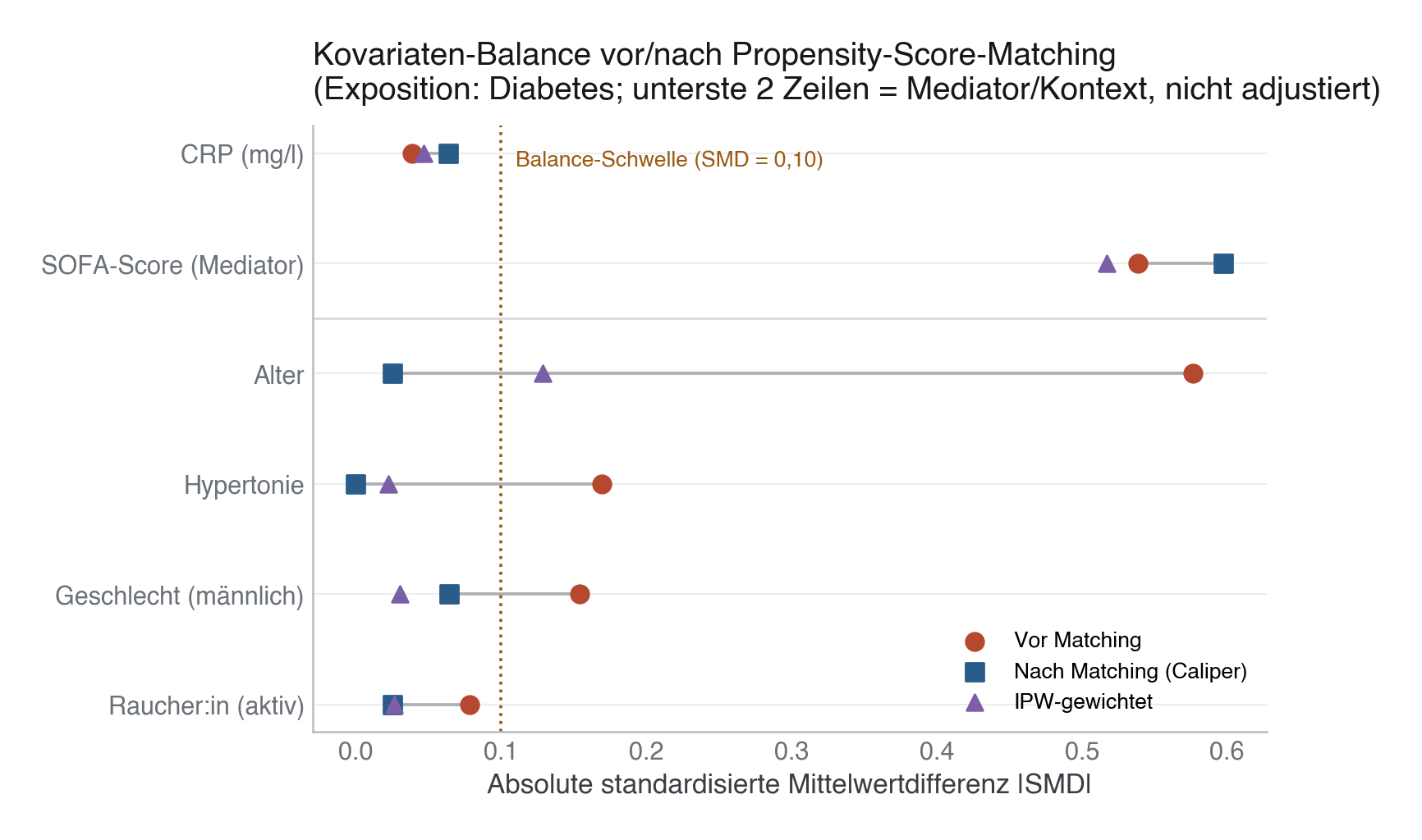
Erzeugt von fig_love_plot() in module/19-propensity-score-causal/code/figures.py, Zeile 44–81.
Python
Python-Code: in eine Datei mit Endung
.py schreiben und mit dem ▶-Knopf in VS Code ausführen – oder Zeile für Zeile in die Python-Konsole. Setzt die in Modul 02 eingerichtete Umgebung voraus.def fig_love_plot(df) -> None: all_covariates = PS_COVARIATES + CONTEXT_COVARIATES before = {v: abs(smd(df[v], df[TREATMENT] == 1)) for v in all_covariates} caliper = 0.2 * df["logit_ps"].std() matched = match_with_caliper(df, caliper) after = {v: abs(smd(matched[v], matched[TREATMENT] == 1)) for v in all_covariates} df = df.copy() df["iptw"] = np.where(df[TREATMENT] == 1, 1 / df["ps"], 1 / (1 - df["ps"])) ipw = {v: abs(smd(df[v], df[TREATMENT] == 1, df["iptw"])) for v in all_covariates} # Order: PS-adjusted covariates first (sorted by pre-matching imbalance), mediator/context last. ordered = sorted(PS_COVARIATES, key=lambda v: before[v]) + CONTEXT_COVARIATES labels = [LABELS[v] for v in ordered] y = np.arange(len(ordered)) fig, ax = plt.subplots(figsize=(7.5, 4.8)) b = [before[v] for v in ordered] a = [after[v] for v in ordered] w = [ipw[v] for v in ordered] ax.hlines(y, [min(x, y2) for x, y2 in zip(b, a)], [max(x, y2) for x, y2 in zip(b, a)], color=SECONDARY, lw=1.4, alpha=0.5, zorder=1) ax.scatter(b, y, color=EVENT, s=60, label="Vor Matching", zorder=3) ax.scatter(a, y, color=PRIMARY, s=60, marker="s", label="Nach Matching (Caliper)", zorder=3) ax.scatter(w, y, color="#7B5EA7", s=50, marker="^", label="IPW-gewichtet", zorder=3) ax.axvline(SMD_THRESHOLD, color="#9A5B12", ls=":", lw=1.3, zorder=2) ax.text(SMD_THRESHOLD + 0.01, 0.96, "Balance-Schwelle (SMD = 0,10)", color="#9A5B12", fontsize=9.5, transform=ax.get_xaxis_transform(), va="top") ax.axhline(len(PS_COVARIATES) - 0.5, color="#D8DADD", lw=1.0, ls="-") ax.set_yticks(list(y)) ax.set_yticklabels(labels) ax.set_xlabel("Absolute standardisierte Mittelwertdifferenz |SMD|") ax.set_title("Kovariaten-Balance vor/nach Propensity-Score-Matching\n" "(Exposition: Diabetes; unterste 2 Zeilen = Mediator/Kontext, nicht adjustiert)") ax.legend(loc="lower right", fontsize=9.5) save(fig, ASSETS / "love_plot_smd.png")