21 · Auswahl der passenden statistischen Methode
dist_anova_vs_kruskal.png
Abbildung · Quellcode
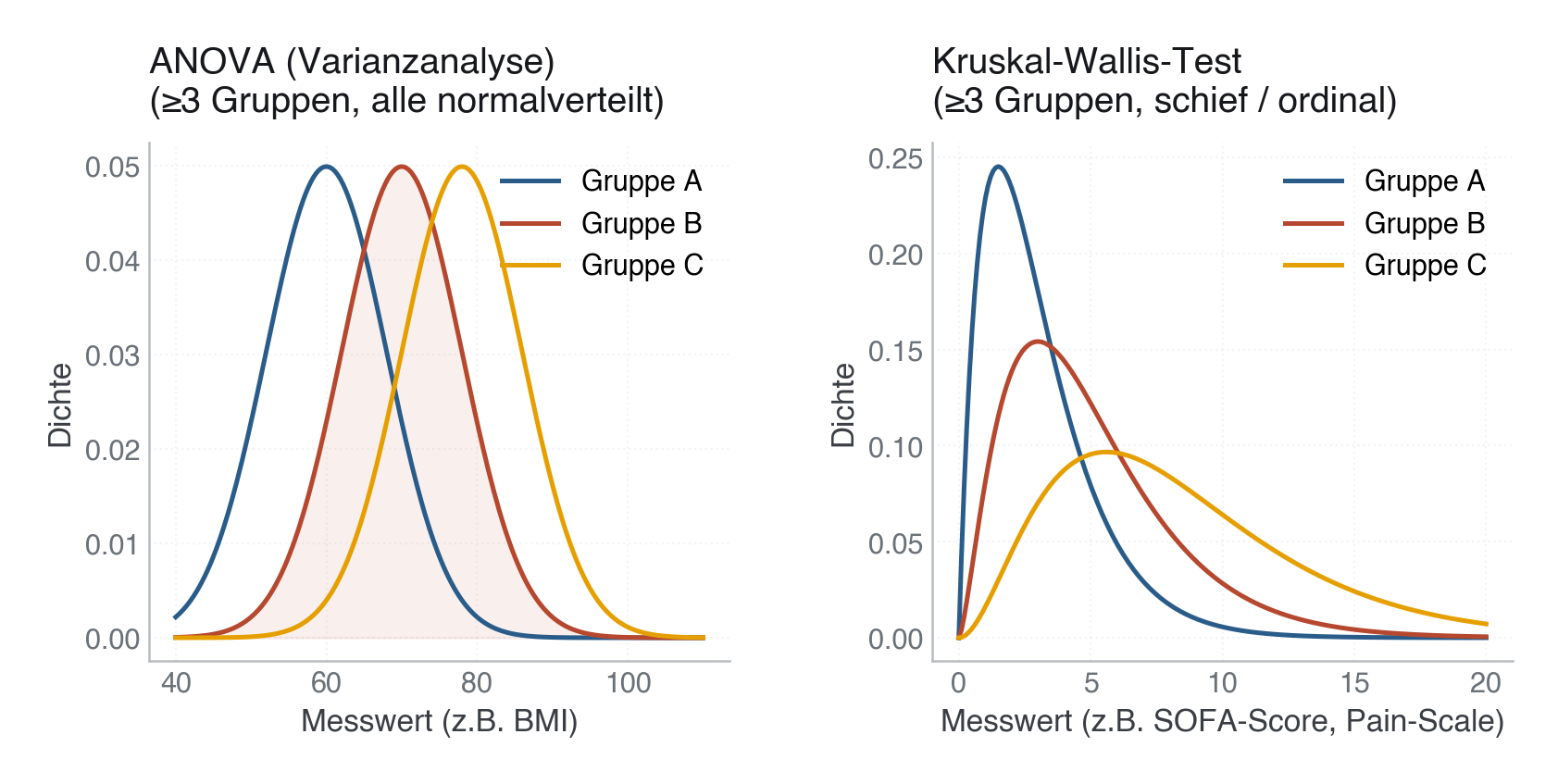
Erzeugt im Abschnitt „dist_anova_vs_kruskal" in data/figures.py, Zeile 826–853.
Dieses Skript läuft von oben nach unten. Der gemeinsame Vorspann — Bibliotheken, Kohorte laden, Plot-Stil — steht am Anfang der vollständigen Datei und gilt für alle Abbildungen darin.
Python
Python-Code: in eine Datei mit Endung
.py schreiben und mit dem ▶-Knopf in VS Code ausführen – oder Zeile für Zeile in die Python-Konsole. Setzt die in Modul 02 eingerichtete Umgebung voraus.# --- 3) ANOVA vs. Kruskal-Wallis --- fig, (ax1, ax2) = plt.subplots(1, 2, figsize=(9.5, 4)) fig.subplots_adjust(wspace=0.35, bottom=0.18) # ANOVA: Three normal curves x = np.linspace(40, 110, 200) ax1.plot(x, stats.norm.pdf(x, 60, 8), color=PRIMARY, linewidth=1.8, label="Gruppe A") ax1.plot(x, stats.norm.pdf(x, 70, 8), color=EVENT, linewidth=1.8, label="Gruppe B") ax1.plot(x, stats.norm.pdf(x, 78, 8), color="#E69F00", linewidth=1.8, label="Gruppe C") ax1.fill_between(x, stats.norm.pdf(x, 70, 8), alpha=0.08, color=EVENT) ax1.set_title("ANOVA (Varianzanalyse)\n(≥3 Gruppen, alle normalverteilt)") ax1.set_xlabel("Messwert (z.B. BMI)") ax1.set_ylabel("Dichte") ax1.legend(loc="upper right") ax1.grid(True, linestyle=":", alpha=0.6) # Kruskal-Wallis: Three skewed curves x_skew = np.linspace(0, 20, 200) ax2.plot(x_skew, stats.gamma.pdf(x_skew, 2, 0, 1.5), color=PRIMARY, linewidth=1.8, label="Gruppe A") ax2.plot(x_skew, stats.gamma.pdf(x_skew, 2.5, 0, 2.0), color=EVENT, linewidth=1.8, label="Gruppe B") ax2.plot(x_skew, stats.gamma.pdf(x_skew, 3, 0, 2.8), color="#E69F00", linewidth=1.8, label="Gruppe C") ax2.set_title("Kruskal-Wallis-Test\n(≥3 Gruppen, schief / ordinal)") ax2.set_xlabel("Messwert (z.B. SOFA-Score, Pain-Scale)") ax2.set_ylabel("Dichte") ax2.legend(loc="upper right") ax2.grid(True, linestyle=":", alpha=0.6) save(fig, M21_DIR / "dist_anova_vs_kruskal.png")