21 · Auswahl der passenden statistischen Methode
dist_paired_t_vs_wilcoxon.png
Abbildung · Quellcode
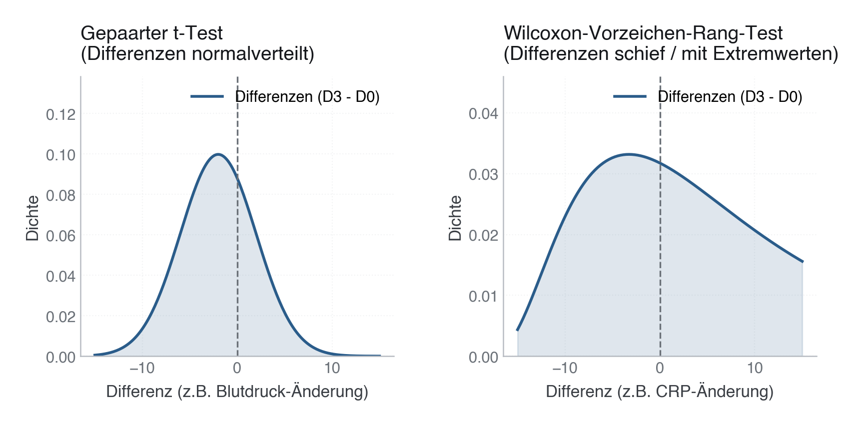
Erzeugt im Abschnitt „dist_paired_t_vs_wilcoxon" in data/figures.py, Zeile 794–824.
Dieses Skript läuft von oben nach unten. Der gemeinsame Vorspann — Bibliotheken, Kohorte laden, Plot-Stil — steht am Anfang der vollständigen Datei und gilt für alle Abbildungen darin.
Python
Python-Code: in eine Datei mit Endung
.py schreiben und mit dem ▶-Knopf in VS Code ausführen – oder Zeile für Zeile in die Python-Konsole. Setzt die in Modul 02 eingerichtete Umgebung voraus.# --- 2) Paired t-Test vs. Wilcoxon Signed-Rank --- fig, (ax1, ax2) = plt.subplots(1, 2, figsize=(9.5, 4)) fig.subplots_adjust(wspace=0.35, bottom=0.18) # Paired t-Test: Normal distribution of differences x = np.linspace(-15, 15, 200) ax1.plot(x, stats.norm.pdf(x, -2, 4), color=PRIMARY, linewidth=2, label="Differenzen (D3 - D0)") ax1.fill_between(x, stats.norm.pdf(x, -2, 4), alpha=0.15, color=PRIMARY) ax1.axvline(0, color=SECONDARY, linestyle="--", linewidth=1.2) ax1.set_title("Gepaarter t-Test\n(Differenzen normalverteilt)") ax1.set_xlabel("Differenz (z.B. Blutdruck-Änderung)") ax1.set_ylabel("Dichte") # Extra headroom above the curve so the legend never crosses the peak. ax1.set_ylim(0, ax1.get_ylim()[1] * 1.32) ax1.legend(loc="upper right") ax1.grid(True, linestyle=":", alpha=0.6) # Wilcoxon: Skewed/heavy-tailed distribution of differences y_skew = stats.lognorm.pdf(x + 20, 0.6, scale=24) # Ensure domain fits bounds ax2.plot(x, y_skew, color=PRIMARY, linewidth=2, label="Differenzen (D3 - D0)") ax2.fill_between(x, y_skew, alpha=0.15, color=PRIMARY) ax2.axvline(0, color=SECONDARY, linestyle="--", linewidth=1.2) ax2.set_title("Wilcoxon-Vorzeichen-Rang-Test\n(Differenzen schief / mit Extremwerten)") ax2.set_xlabel("Differenz (z.B. CRP-Änderung)") ax2.set_ylabel("Dichte") # Extra headroom above the curve so the legend never crosses the peak. ax2.set_ylim(0, ax2.get_ylim()[1] * 1.32) ax2.legend(loc="upper right") ax2.grid(True, linestyle=":", alpha=0.6) save(fig, M21_DIR / "dist_paired_t_vs_wilcoxon.png")